ML-fundamentals
An overview of machine learning
Terminology
- general intelligence: stuff like humans, biological intelligence at the level of humans
- artificial intelligence: when a machine can perform a task as good or better than a human can, like classifying images.
- data: tabular data or data that can be stored in a single file
- big data: data that is too large to be stored in a tabular format, so it's stored in a stream instead.
- AGI: when artificial intelligence achieves the capability of general intelligence, when AI becomes better at tasks than most humans are.
- Strong AI refers to machines that display full human-like intelligence, including emotions, creativity, and a sense of purpose—like the intelligent characters you see in science fiction. It's the idea of a machine that truly thinks and understands like a person, but this is still mostly theoretical today.
- Weak AI, on the other hand, is designed for specific tasks. It can process language or recognize patterns but doesn't actually understand or have consciousness. For example, Siri is a weak AI—it listens to your questions and matches them to programmed responses without real understanding.
- predictive AI: regression, classification, or clustering tasks, which is a type of AI that analyzes large amounts of data to find patterns and make predictions about future behavior
- generative AI: generates content
Big data
Bid data satisfies the three Vs:
- Volume: high volume of data, at least several terabytes
- Velocity: high influx rate of data, like 100 megabits per second
- Variety: high variety arising from a complex data structure storage like audio, stream, or image data.
When dealing with Big Data, you arive at the CAP theorem from system design, where there is a tradeoff between consistency, availability, and partitioning with trying to replicate data across multiple machines.
Weak AI vs Strong AI
Machine learning is weak AI, where we use mathematical techniques like statistics or hardcoded rules to learn patterns in data.
- early weak AI: hardcoded rules designated by experts, much like a hardcoded decision tree
- modern weak AI: learning patterns via computational statistic inference and gradient descent, where a function hypothesis is approximated computationally instead of cognitively.
Alignment
The mismatch between what the AI does and what humans actually want is called the alignment problem, which is what happens when an AI might do exactly what it's programmed to do but in a way that humans don't expect or want.
The alignment problem arises when you program an AI to do a task and you assume that it will think and reason like a human on that same task without implementing guardrails or thinking it through better.
It's a key ethical issue because AI systems can make many decisions quickly, and if they're not aligned with human values, they might cause harm without anyone noticing right away.
There are 4 alignment problems in AI:
- value alignment: Value alignment in AI refers to the challenge of ensuring that an AI system's actions match human values and intentions
- traceability: Decision traceability in AI refers to the challenge of understanding how an AI system arrives at its decisions.
- Many AI systems, especially those analyzing massive datasets, act like a "black box"—they produce results based on complex patterns that are nearly impossible for humans to fully trace or explain.
- copyright: Copyright law protects original human-created content, but there is ongoing debate about whether using such content to train AI models qualifies as fair use.
- privacy: Privacy in the U.S. is often governed by flexible guidelines rather than strict rules, allowing companies to collect and use personal data extensively.
Value alignment
For example, if an AI system is designed to reduce health insurance costs by targeting high-cost customers, it might cancel policies for older people to save money, which is not the intended ethical outcome.
Types of machine learning
Supervised learning
Supervised learning is based on known feature data and known labels , where is the unknown, true function that provides a 100% deterministic, correlated relationship between and .
The goal of supervised learning is to estimate this true relationship using an approximation function to make predictions , and then based on the error between prediction and expected known label , we tune the hypothesis function to grow closer to the true by trying to minimize error as much as possible
The closer is to , the better the model performs, which means that hypothesis that minimizes the error (the discrepancy between the hypothesis function and the true unknown function) the most, is the best hypothesis possible, accounting for initial assumptions and bias.
Basically, the goal is to minimize something like this:
Where is some loss function calculating the prediction error for the th training sample , and is some cost function that aggregates the losses.
- loss: the prediction error for one training sample and its expected known value
- cost: the total prediction error over all training samples, found via aggregating losses.
Semantic gap in machine learning
The semantic gap refers to the difference between the data we have and the actual information or meaning we want to extract from it.
In machine learning, this often means that the features or data available (like photographs) do not fully capture the true characteristics that distinguish what we want to classify (such as the difference between cats and dogs).
NOTE
Basically a semantic gap occurs when the features you have don't explain the data 100%, and there are some other hidden variables you can't account for, and we just approximate through machine learning.
For example, a photo contains visual information, but it doesn’t include deeper properties like DNA, bone structure, or behavior, which are essential to truly distinguish a cat from a dog. The machine learning model tries to bridge this gap by finding patterns in the available data, but it is limited to what is present in the data. Sometimes, the model may pick up on irrelevant features (like snow in the background of dog photos) rather than the actual distinguishing features.
The semantic gap highlights the challenge that the data used for training may not be sufficient or relevant enough to solve the real-world problem accurately.
Features

Univariate data and bivariate data
In statistics, the terms univariate and bivariate refer to the number of variables being analyzed.
-
Univariate data involves the analysis of a single variable. The goal is to describe the distribution of this variable, often using measures of central tendency (like mean or median) and measures of spread (like variance or standard deviation).
-
Bivariate data involves the analysis of two variables simultaneously. The goal is to understand the relationship or correlation between these two variables.
Univariate data and feature types
There are 4 types of univariate data, meaning when you're looking at just one feature:
- nominal data : categorical data with no order to the data
- ordinal data : categorical data with order to the data and labels
- continuous data : numerical data that includes decimals
- discrete data : numerical data that includes only integers or a finite collection of integers.
There are two types of feature types:
- qualitative: either nominal or ordinal data, where the feature is based on categories and uses one-hot encoding to encode the category numerically.
- quantitative: either continuous or discrete data, using numerical data.
Measures of central tendency
Based on the skewness of the distribution, these facts are guaranteed:
- Symmetric : mean = median
- Right skewed : mean > median
- Left Skewed : mean < median
Best measures of central tendency for each situation
- Median : when dealing with ordinal data or with skewed data
- Mean : When dealing with evenly distributed data like in a normal distribution
Measures of spread
- variance : we can use the
np.var(arr)method to get the variance of the data within a vector. - standard deviation : we can use the
np.std(arr)method to get the standard deviation of the data within a vector. - coefficient of variation : the coefficient of variation is the standard deviation divided by the mean.
x = np.random.randn(20)

print("standard deviation:", np.std(x))
print("variance:", np.var(x))
print("coefficient of variation", np.std(x) / np.mean(x))
Feature scaling
Most machine learning algorithms use distance metrics (like Euclidean distance) or gradient descent for optimization.
If one feature has a range of 0-1 and another has a range of 0-1,000,000, the algorithm will be dominated by the larger magnitude feature, even if the smaller feature is more predictive. That is why we must scale feature ranges into a more suitable, standardized and smaller range.
So why do we use feature scaling? Three key principles:
-
Comparability: It brings all features to a similar scale, making them directly comparable.
-
Convergence: Algorithms that use Gradient Descent (like Logistic Regression or Neural Networks) converge much faster when features are scaled.
-
Distance Sensitivity: Algorithms like KNN, K-Means, and PCA are highly sensitive to the magnitude of features.
There are three types of scaling:
- Standardization (Z-score normalization): Transforms data to have a mean of 0 and a standard deviation of 1. It is robust to outliers compared to Min-Max scaling.
- Normalization (Min-Max Scaling): Rescales the data to a fixed range, usually 0 to 1. It is very sensitive to outliers (a single outlier can compress all other values into a tiny range).
- log 10 scaling: Simple rescaling of data on large magnitudes, but not actually used to improve the performance of a machine learning model in the sense of how feature scaling is supposed to be. It's only used for human-readable values so we can see smaller values instead of all values being in the thousands.
from sklearn.preprocessing import StandardScaler, MinMaxScaler
import numpy as np

# Sample data: [Feature A, Feature B]
data = np.array([[10, 0.001], [20, 0.002], [30, 0.005], [1000, 0.01]])

# Standard Scaler
std_scaler = StandardScaler()
std_data = std_scaler.fit_transform(data)

# Min-Max Scaler
mm_scaler = MinMaxScaler()
mm_data = mm_scaler.fit_transform(data)

print("Original Data:\n", data)
print("\nStandard Scaled (Mean=0, Std=1):\n", std_data)
print("\nMin-Max Scaled (Range 0-1):\n", mm_data)
Log transformation
We use log transformation to get better resolution on a plot where our data varies widely between magnitudes, like on a range from 1,000 - 350,000.
np.log10(arr): applies base 10 log to all elements in the array. Returns new arraynp.log(arr): applies natural log to all elements in the array. Returns new array
We want to apply the log 10 transformation on our features that vary widely in magnitude.
Min-max scaling
Rescales the data to a fixed range, usually between 0 to 1.
- pro (fixed range): a fixed range offers predictability and standardization in mathematical outputs
- con (sensitive to outliers): very sensitive to outliers since a single outlier can compress all other values into a tiny range.
- For example if the max is 1,000,000 and the average is maybe 29, then that single million value outlier basically ruins the rest of the range because it makes every single other value extremely small while the largest value is equal to 1.
Standard scaling
Standard scaling fits features to a normal distribution, making each feature have a mean and a standard deviation
The formula for standard scaling is this, where you subtract the mean from each feature value, and then divide that by the standard deviation.
This results in each scaled feature having a mean = 0 and standard deviation = 1.
NOTE
This is the exact same thing as the Z-score. It returns the z-score of each feature value, about how many standard deviations the observation is from the mean.
WARNING
If you try to calculate the coefficient of variation on standard scaled data, then you will get an error because standard scaled data always has a mean = 0 and variance = 1, thus 1 / 0 nets you undefined.
We can get access to a standard scaler through the sklearn library, like so:
from sklearn.preprocessing import StandardScaler as SS
standard_scaler = SS()
ss.fit_transform(df): takes in a dataframe or another 2D array, and then feature scales all the feature columns. It returns the scaled dataframe or array.ss.fit(df): calculates mean and standard deviation of data and stores it in thessobject. ReturnsNoness.transfom(df): feature scales the data after you callss.fit(). Only does this for standard scaler, but applies fitted parameters to data
These three methods do different things depending on which object instance of sklearn you use. Here is how they work in general:
.fit(): fits the data to the model.transform(): transforms the model.fit_transform(): fits the data to the model, and then returns the transformed data.
standard_scaler = StandardScaler()
scaled_df = standard_scaler.fit_transform(data)
Feature importance
Feature importance matters because you want to find the most important features that contribute the most to a target value, as focusing on those features will make your predictor stronger.
Here are the core benefits
- improves performance, reduces model complexity: It helps you focus on the most relevant data, improving prediction accuracy and reducing model complexity.
- improves explainability: lowering the number of features makes explainign those features and thus improves model interpretability.
Feature engineering
Feature engineering is the process of creating new features from existing raw data and other existing features to use new features that would benefit the model training in order to improve a model's performance
NOTE
Good feature engineering makes the difference between an average model and an excellent one, as it helps the model to focus on the most relevant patterns in the data.

Here are examples of common feature engineering tasks to create, modify, or delete features for facilitating better input data to the model:
- combining existing features together: you can achieve a lower complexity model (and thus less variance) by making the data lower complexity by combining several features into one single, powerful predictive feature.
- removing highly correlated features: features that are highly correlated with each other will be redundant. Therefore removing them lets you make your model simpler.
- impute missing data: features with missing data are bad data, so it's better to fill them via imputation or remove the feature entirely.
Imputation
Imputation is the process of filling in missing data values in your dataset so that your machine learning model can train effectively.
Instead of leaving gaps or incomplete information, imputation estimates those missing values based on other data, ensuring the dataset is complete and consistent.
NOTE
Imputation is important because most models require complete data to learn patterns accurately, and imputation allows you to infer reasonable estimates for missing data instead of throwing it away.
Data preparation
Data analysis
Here are basic data analysis tools you can do:
- verify which features have missing values: it's important to understand which features may have null values
# Verify which features have missing values
housing_df.isnull().sum()

# Calculate the % of missing data
housing_df['total_bedrooms'].isnull().sum()/housing_df.shape[0] * 100
- find most important features: use pandas to find feature importances
# Determine feature importance - random forest algorithm is that it gives you the ‘feature importance’ for all the variables in the data
# plot the 6 most important features
plt.figure(figsize=(10,6))
feat_importances = pd.Series(rf_model.feature_importances_, index = X_train.columns)
feat_importances.nlargest(6).plot(kind='barh');
Data preparation
One-hot encoding
One-hot encoding is the process of converting text enum data into numerical data, where if an enum is of cardinality , then the one-hot encoded vector of a datum of that enum will be of dimensionality , where one value 1 and all other values are 0.
That one position where the value is 1 corresponds to that datum's position in the enum, meaning that one-hot encoded vector representation uniquely represents that enum.
pd.get_dummies(housing_df['ocean_proximity'])
Training, Validation, Test
Generalization error
Generalization error is how much your model errors on new data it hasn't seen before.
NOTE
Therefore, to get an accurate view of how your model is doing, you need to make sure that you cannot reuse a training set as your test set when doing the generalization error. You must calculate the generalization error on new data that you haven't seen before, otherwise you introduce biases in the data.
Let's take a look at training performance vs generalization performance:
- in-sample performance: when training on a train set, which we use to iteratively find a good hypothesis, the error on the training set will be optimistic and having fit the model to the training set, the model would be biased to performing well on the training set.
- out-of-sample performance: When training on new data, the model has never seen before, it can't use its underlying biases to get a lower error, and therefore is a more accurate depiction of a model's performance
- overfitting: When we overfit a data set, essentially the model does well on the training data but fails to generalize on the testing data. It means training score is less than testing score.
- underfitting: When we underfit a data set, it performs poorly on both the training set and and test set.
- internal validity : how well the model performs on the training data
- external validity : how well the model performs on the test data
Train test-split
The performance on the validation and test sets will be roughly the same, but the test set will be slightly worse since you will not have trained on the test set at all.
- train set: The dataset partition which you use to train your model - around 60% of dataset
- validation set: The dataset partition which you use to choose the best hyperparameters for your model - around 20% of dataset
- test set: The dataset partition which you use to test your model - around 20% of dataset
validation is the process of evaluating a model on data that it hasn't been trained on yet.

The validation set is a portion of the dataset with the purpose of evaluating how well the model would perform on new unseen data.
NOTE
The reason why the test set can only be tested once is because if you test on it multiple times, you're essentially just using the test set as a validation set and you're fitting to it.
sklearn implementation
Here is an example of how we can do in sklearn:
The tts() method takes in an array of features and an array of target data, and then returns an array of 4 nested arrays, representing the training data and testing data respectively.
from sklearn.model_selection import train_test_split as tts

X_train, X_test, y_train, y_test = tts(x, y, test_size=0.2, shuffle=True, random_state=201)
The first two arguments you pass to the tts() method are the array of features, x, and the array of target values y. Then after that here are the kwargs you can supply:
test_size=: the percentage of data to allocate to testing. 20% is pretty good here.shuffle=: whether to randomly sort data or not.random_state=:int. a random seed to set so that you get back the same split every time.
k-fold cross validation
The idea of K-fold validation is to make each batch of data as the testing data so that there are no discrepancies and bias between what we're choosing for training data and testing data.
You will make models during this process.
- Split data into equally sized groups, called folds
- Use the first fold as a validation fold, which is the testing data, and then merge the rest of the folds into a group as the training data, called train folds.
- Move on to make the second fold as the validation fold, and then merge the rest of the folds into a group as the training data.
- Continue this process for iterations, covering all folds, and then compute the error for each iteration
- The total error is the average of all error yields.
In total, each fold will be in the training data times and in the testing data 1 time. Per iteration, you have train folds and 1 validation fold.

NOTE
K-fold cross validation provides a more robust estimate of the model's true performance and helps detect underfitting or overfitting.
Theory of k
The value of has a bias-variance tradeoff.
- As the number of folds increases, You do better on training data and do worse on testing data (testing data is a smaller portion of data) and thus variance increases
- As the number of folds decreases, You do worse on training data and do better on testing data (testing data is a bigger portion of data, and you're training on less of data) and thus bias increases
kfold in code
-
Import
kfoldfrom sklearn.model_selection import KFold -
Create a kfold instance from the
KFoldclasskf = KFold(n_splits = 10, random_state=146, shuffle=True) -
Use the
kf.split(data)method to create kfold splits on your data, which should be a 2D array. This method returns a generator, so you should iterate through itfor idxTrain, idxTest in kf.split(x):Xtrain = x[idxTrain]Xtest = x[idxTest]ytrain = y[idxTrain]ytest = y[idxTest]
And here's a convenience method:
from sklearn.model_selection import KFold

def do_Kfold(model,X,y,k,scaler = None, random_state = 146):

    kf = KFold(n_splits=k, random_state = random_state, shuffle=True)

    train_scores = []
    test_scores = []

    for idxTrain, idxTest in kf.split(X):
        Xtrain = X[idxTrain, :]
        Xtest = X[idxTest, :]
        ytrain = y[idxTrain]
        ytest = y[idxTest]
        if scaler != None:
            Xtrain = scaler.fit_transform(Xtrain)
            Xtest = scaler.transform(Xtest)

        model.fit(Xtrain,ytrain)

        train_scores.append(model.score(Xtrain,ytrain))
        test_scores.append(model.score(Xtest,ytest))

    return train_scores, test_scores
Leave-one-out-validation
Leave one out validation is where you train on every single observation except for one, which is your test set.
NOTE
This is extremely useful when paired with K nearest neighbors.
Grid Search
Here are the essential components to grid search:
- estimator : the model to run grid search on
- param grid : the dictionary of hyperparameters to try and optimize
- cv : the KFold validation and number of folds to use
- scoring: how the Grid model shoudl evaluate performance to select the best estimator.
Grid search kwargs
cv=: the custom cross validation to use, like a custom KFold instance. By default it's 5 folds KFold validation.scoring=: string, how the Grid model should evaluate performance to select the best estimator."accuracy": uses accuracy as the score. Useful for classification"neg_mean_squared_error": uses negative mean squared error as score. Useful for regression"recall": uses recall as the score
sklearn implementation
from sklearn.model_selection import KFold, GridSearchCV
from sklearn.ensemble import RandomForestClassifier as RFC

# 1. create parameter grid
param_grid = {
    'n_estimators' : [64, 100, 128],
    'max_depth' : [2,3,4,5],
    'min_samples_split' : [2,3,4,5]
}

# 2. create custom cv validation
cv = KFold(n_splits=10, random_state=146, shuffle=True)

# 3. create estimator
estimator = RFC()

# 4. create grid search
grid = GridSearchCV(estimator, param_grid, cv=cv, scoring='accuracy')

# 5. train grid
grid.fit(Xtrain, ytrain)
Overfitting, Underfitting, Bias vs Variance
Overfitting vs Underfitting
When we overfit a data set, essentially the model just well on the training data but fails to generalize on the testing data. It means training score is less than testing score.
When we underfit a data set, it performs poorly on both the training set and and test set.
- internal validity : how well the model performs on the training data
- external validity : how well the model performs on the test data
- overfitting: high internal validity, low external validity
- underfitting: low internal validity, low external validity
How model complexity affects performance
Model complexity affects performance because either your model is too complex and thus "memorizes" the training data while failing to generalize, or the model is too simple to capture any complex pattern in the data.

- low complexity: low complexity models can't lean complex patterns
- high complexity: high complexity models memorize patterns in data, but may not generalize.
We quantify the number of candidate hypotheses in the hypothesis set by degrees of freedom, also known as VC dimension. So degrees of freedom is just the cardinality of the hypothesis set.
- small VC dimension: We may not even have a good hypothesis in the hypothesis set since it's so small, which is a symptom of choosing a simple model.
- large VC dimension: Although it is likely we contain a good hypothesis somewhere in the hypothesis set, it's harder to find, which is a symptom of choosing an overly complex model.
NOTE
VC dimension in a nutshell
VC dimension is a way to quantify the complexity of a model, and mathematically it represents the cardinality of the hypothesis set.

NOTE
Overfitting in a nutshell
Overfitting is a symptom of having a too complex model for the data, leading to the model fitting the noise and thus overperforming on training data but failing to generalize to testing data.
From model complexity we get bias and variance:

- bias: how limited or inflexible a model's assumptions are.
- high bias: You have high bias when the model is low in complexity, like a linear model, because it makes a grand assumption that the data follows a linear pattern.
- low bias: You have low bias when the model is high in complexity, like a 100 degree polynomial, because it can adapt itself to a model any degree lower than itself. It has no assumptions of what the data pattern actually looks like, it can fit itself to whatever the underlying pattern is, as long as the initial model's degree of freedom are high enough.
- variance: a measure of how much a model's predictions would change if it were trained on different subsets of the training data. In other words, it's the cardinality of the hypothesis set.
- high variance: You have high variance when the model is high in complexity, because high complexity models are very sensitive to small changes in the training data because they contort themselves to memorize the data, changing the hypothesis wildly for different trainind set.
- low variance: You have low variance when the model is low in complexity, because low complexity models like linear models produce more consistent predictions across different training sets.

There's a tradoff between bias and variance.
- As model complexity increases:
- bias decreases, because a more complex model can capture more complex patterns and assumes less.
- variance increases, because a more complex model means that it is more sensitive to change when trained on different data sets.
- As model complexity decreases:
- bias increases, because a less complex model has more rigid assumptions.
- variance decreases, because a less complex model is less sensitive to change when trained on different data sets.
Learning curves
We can see if a model is overfitting or underfitting by plotting a learning curve, which plots the model accuracy/performance on the y-axis against the number of training examples on the x-axis.

From the learning curve, we can see how to mitigate overfitting and improve performance:
- get more training data: When we have more training data, it is less likely that by chance we choose the wrong hypothesis function.
- regularization: to prevent fitting to too much noise, making a complex model simpler.
Bias-variance tradeoff
- low VC-dimension: simple models have high bias and low variance, thus they underfit.
- high bias: the chance of finding the best hypothesis in the set is high.
- low variance: Since the VC dimension is low, there are not many variations of the hypothesis and thus not much of a chance of finding a better, more complex model.
- high VC-dimension: complex models have low bias and high variance, thus they overfit.
- low bias: the chance of finding the best hypothesis in the set is low, since it's such a small subset of the hypothesis set.
- high variance: There are many variations of hypotheses, and even training on one different sample can lead to many different hypothesis functions in this set.

This is a fitting graph, which plots model error on the Y-axis and VC-dimension on the X-axis:

How noise affects overfitting
Noise refers to random variations or errors in data that don't represent true underlying patterns like random fluctuations in sensor readings or errors in data

Noise is often impossible to remove, but our goal is to find the best model that finds the pure 100% signal of the pattern, ignoring noise, which is a perfect fitting of the data.
- Overfitting occurs when a machine learning model learns the noise in the patterns rather than the signal of the underlying pattern, and it has two core causes:
- Not enough data: not enough data to reduce overfitting on the learning curve
- High model complexity: model is too complex
- Underfitting occurs when a machine learning model has high bias, meaning it's too simple to capture the underlying pattern of data.
 .
Dimensionality
Dimensionality of your data is the number of features that contribute to the data.
Curse of dimensionality
The curse of dimensionality states that:
As the dimensionality increases, the number of data points required for good performance of any machine learning algorithm increases exponentially.
The cure of dimensionality has many effects:
- equidistant points: high-dimensional points are sparse and spread out, thus distance-based algorithms like KMeans or KNN degrade in utility with high dimensionality.
- harder to learn patterns: as the set of all possible data points becomes increasingly more sparse, it becomes harder to learn patterns in the data.

Dimensionality Reduction
Dimensionality reduction is the practice of approximating high dimensional data to lower dimensions while trying to maintain as much accuracy and capture most of the patterns in the original data as possible.

Lower dimensionality brings us two key benefits:
- easier to understand and visualize: As humans, we can't visualize past 3 dimensions.
- easier to train: most models perform better on low-dimensional data.
SVD for dimensionality reduction
PCA for dimensionality reduction
PCA finds the directions (axes/vectors) in which the most variance the data set is retained, and those directions are called principal components

- The first principal component, also called PC1, accounts for the highest percentage of variance in the data set (it's the most important feature)
- Each succeeding principal component will be orthogonal to the previous PC, and explain less and less variance.
tSNE for dimensionality reduction
Feature cardinality
Cardinality of a feature refers to how many unique values that feature has.
High cardinality features can increase the complexity of models, particularly those based on tree algorithms.
- how high cardinality affects decision trees: Decision trees, for example, may struggle to effectively split on high cardinality features, leading to inefficient use of computational resources and potentially overfitting.
For features with a high cardinality, more data is the cure to improve model performance.
univariate linear regression
Understanding how univariate linear regression works will give you a foundational base to understand every other machine learning model out there.
Algebraic formulation
Model and cost
To model , we want to find a function (this notation means that is variable while and are fixed parameters) that is a good approximation for that line.
We use cost and loss:

For this, we need to know what to minimize/optimize:
- loss: let the loss function be squared error
- cost: let the cost function be mean squared error
So our goal is this:
There is also alternative notation:
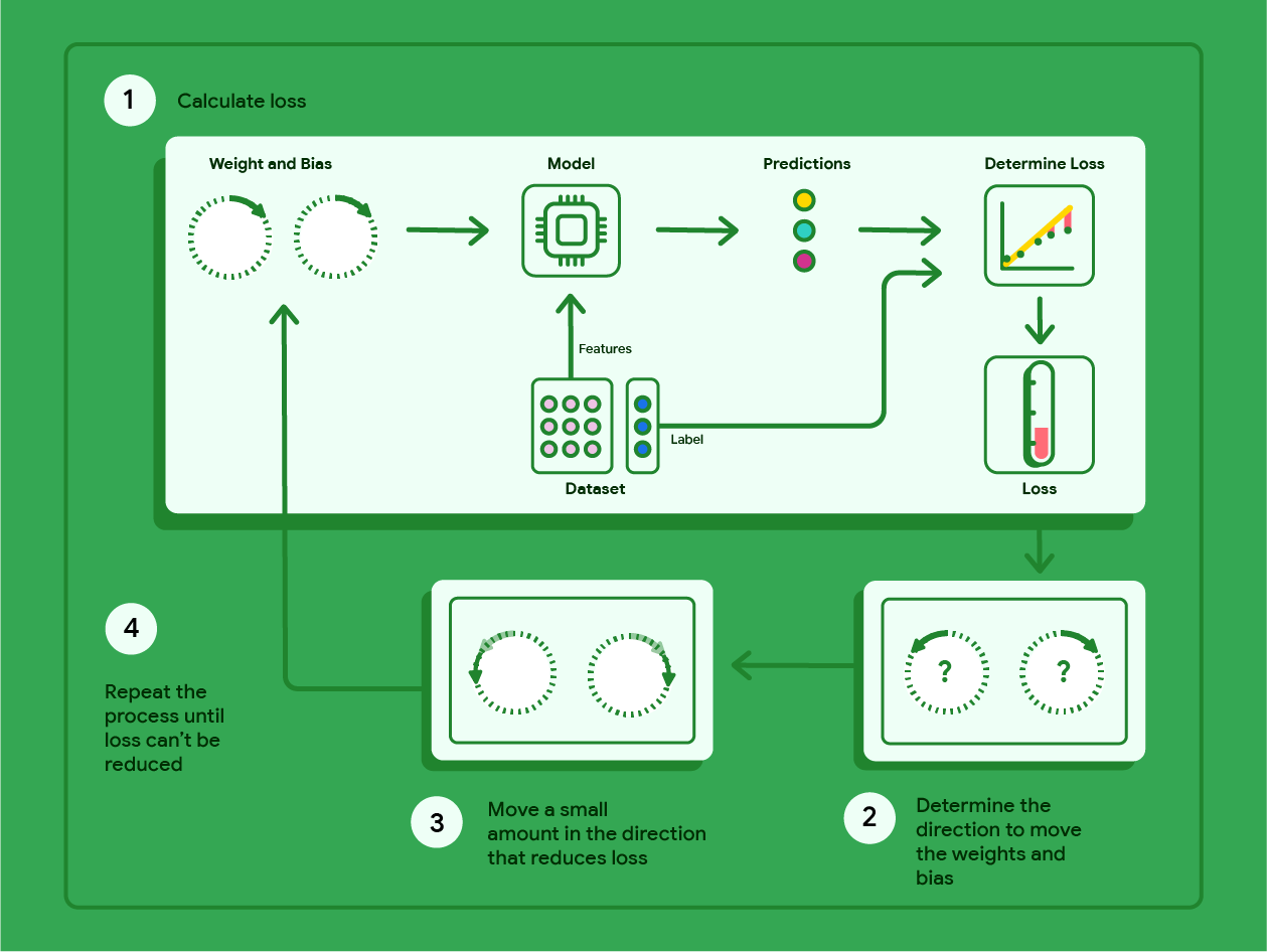
Gradient descent
For a single training sample, we calculate .
We then want to calculate the gradient of loss with respect to parameters and to figure out how to change those parameters.
- Calculate loss or cost
- Calculate gradient with respect to loss or cost
- Perform gradient descent update with a decently small learning rate
- Repeat this process until an update of the previous iteration is very small.
Gradient descent basics
Here's some basic terminology concerning gradient descent:
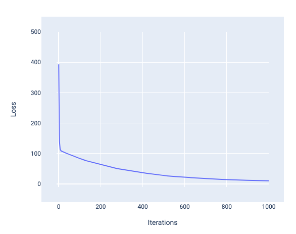
- loss curve: plotting cost against number of iterations to view the "elbow" of diminishing returns for when to stop gradient descent.
- learning rate: a percentage multiplier quantifying the proportion of the gradient to step down.
Loss curve
When training a model, you'll often look at a loss curve to determine if the model has converged. The loss curve shows how the loss changes as the model trains.
The following is what a typical loss curve looks like:
- y-axis: Loss is on the y-axis
- x-axis: iterations are on the x-axis
Learning rate
Learning rate is a floating point number you set that influences how quickly the model converges.
- If the learning rate is too low, the model can take a long time to converge.
- However, if the learning rate is too high, the model never converges, but instead bounces around the weights and bias that minimize the loss.
The difference between the old model parameters and the new model parameters is proportional to the slope of the loss function multiplied by the learning rate.
Batches, epoch, gradient descent types
- batch: a small portion of a dataset
- batch size: Batch size is a hyperparameter that refers to the number of examples the model processes before updating its weights and bias
- iteration: a computational procedure concerning a single batch
- epoch: completion of one iteration of gradient descent on the batch size
You might think that the model should calculate the loss for every example in the dataset before updating the weights and bias.
However, when a dataset contains hundreds of thousands or even millions of examples, using the full batch isn't practical.
That's what gives us multiple types of gradient descent:
| Type | Speed | Stability | Has vectorization? |
|---|---|---|---|
| Batch gradient descent | Slow | Highest, completely stable | Yes |
| Stochastic gradient descent | Fastest | Lowest stability, noisy, but moves generally downhill. | No |
| Mini-batch gradient descent | Fast | Medium stability | Only a bit |
- Batch gradient descent: each step of gradient descent vectorizes over all the training examples to calculate the gradient with respect to cost.
- stochastic gradient descent: each step of gradient descent chooses only one random training sample to calculate the gradient with respect to cost.
- mini-batch gradient descent: each step of gradient descent chooses a small randomly sampled batch of training sample to calculate the gradient with respect to cost.
Batch gradient descent
Batch gradient descent is where each step of gradient descent uses all the training examples to calculate the gradient with respect to cost.
NOTE
This is what people usually think of by gradient descent.
- con - slow: This is more computationally expensive because you’re training on the entire dataset at once, where each gradient descent step computes on the entire dataset.
- pro - accurate: but it has the most stable downhill gradient descent since you KNOW that you’re going in the opposite direction of the correct gradient.
- pro - uses vectorization: Benefits from vectorization
WARNING
TIP: Batch gradient descent is no longer feasible or efficient after N >> 1, meaning you have more than 1,000,000 training samples.
Stochastic gradient descenet
stochastic gradient descent is where you train on one random training sample at a time for the feed forward and backprop process, and update parameters based on one training sample per iteration.
It is the fastest form of gradient descent, but most unstable since you’re basing entire parameter update off of one training sample
Here are the pros:
- Quick and computationally efficient
Here are the cons:
- Does not benefit from vectorization
- noisy descent
Mini-batch gradient descent
Mini-batch stochastic gradient descent is a compromise between full-batch and SGD.
mini batch gradient descent is where you train on a small randomly sampled batch of training samples for the feed forward and backprop process and update parameters based on calculation from that batch.
Here is the exact formalism 1. For number of data points, the batch size can be any number greater than 1 and less than . 2. The model chooses the examples included in each batch at random, averages their gradients, and then updates the weights and bias once per iteration.
Determining the number of examples for each batch depends on the dataset and the available compute resources. In general, small batch sizes behaves like SGD, and larger batch sizes behaves like full-batch gradient descent.
TIP
A batch size of 100 training samples per iteration is the most recommended
Epochs
In general, more epochs produces a better model, but also takes more time to train.
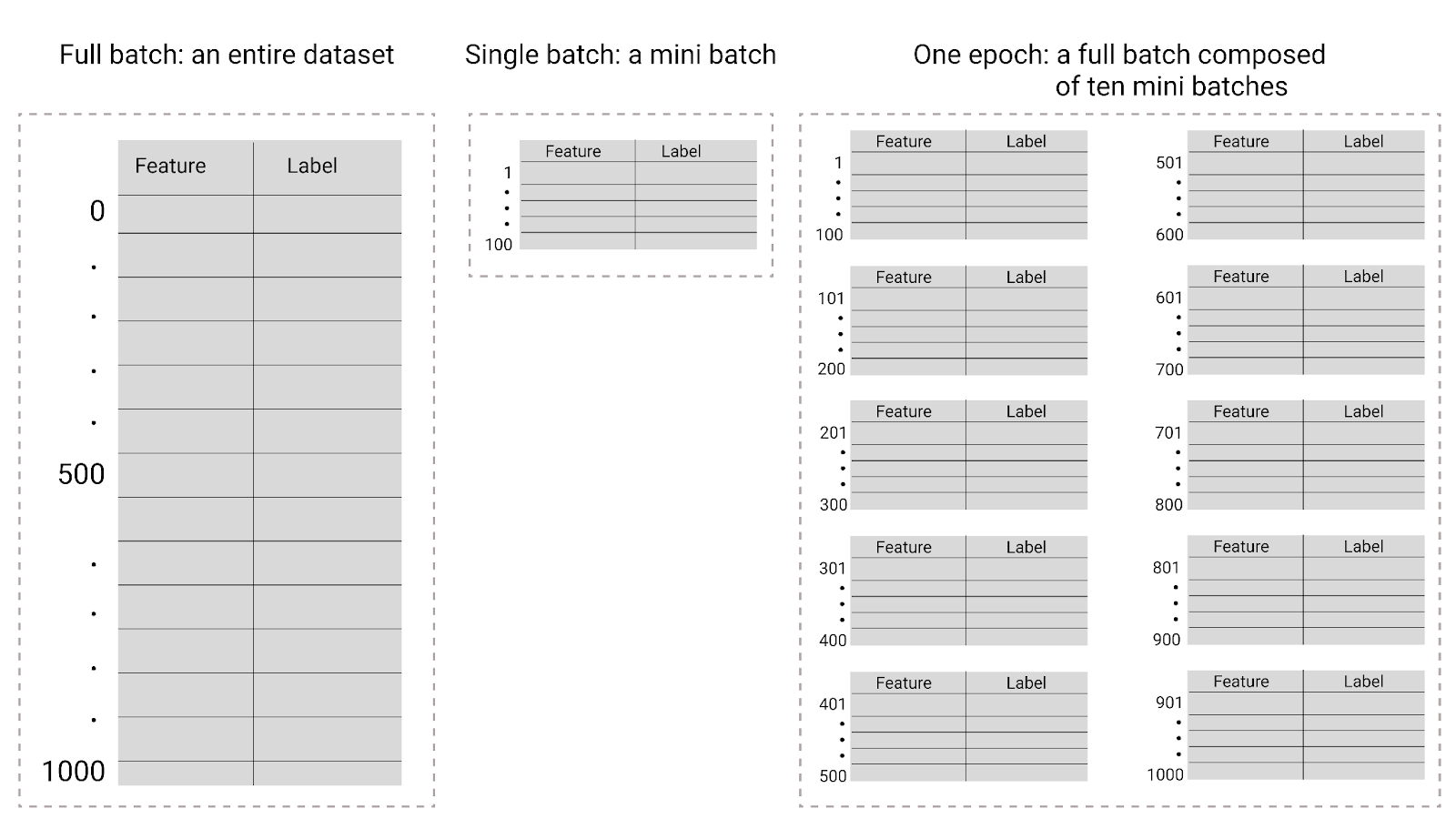
| Batch type | When weights and bias updates occur |
|---|---|
| Full batch | After the model looks at all the examples in the dataset. For instance, if a dataset contains 1,000 examples and the model trains for 20 epochs, the model updates the weights and bias 20 times, once per epoch. |
| Stochastic gradient descent | After the model looks at a single example from the dataset. For instance, if a dataset contains 1,000 examples and trains for 20 epochs, the model updates the weights and bias 20,000 times. |
| Mini-batch stochastic gradient descent | After the model looks at the examples in each batch. For instance, if a dataset contains 1,000 examples, and the batch size is 100, and the model trains for 20 epochs, the model updates the weights and bias 200 times. |
Evaluating the model
Coefficient of determination
We need some way to evaluate how well our model does and you can do that either with loss or something in statistics called the coefficient of determination, which only works in two-dimensional data (features X and output y).
- coefficient of determination: denoted via , and has bounds .
- use case: used as a measure of correlation strength between two variables
- correlation coefficient: denoted by , which is just the square root of the coefficient of determination, and has bounds .
- use case: used as a measure of correlation strength
NOTE
The null model is just predicting the mean, which means that the null model has an value = 0
Null model
In linear regression, the Null Model is the simplest possible baseline. It assumes that the features () have no predictive power, so it simply predicts the mean () of the target variable () for every observation.
- Equation:
- Purpose: It serves as a benchmark. If your regression model isn't better than the null model, your features are not useful.
The null model will just predict that every point is equal to the mean, giving a straight line. Then from there, we can get the coefficient R^2, which is the coefficient of determination.
You can also think of it like this:
Sci-kit Learn Linear Regression
Here is a basic pipeline:
- Create data set, preprocess it
import sklearn
from sklearn.model_selection import train_test_split

# remove spaces from column names and convert all to lowercase and remove special characters as it could cause issues in the future
housing_df_encoded.columns = [c.lower().replace(' ', '_').replace('<', '_') for c in housing_df_encoded.columns]

# Split target variable and feature variables
X = housing_df_encoded[['housing_median_age', 'median_income','bedrooms_per_room','population_per_household','coords','ocean_proximity__1h_ocean',
                        'ocean_proximity_inland','ocean_proximity_island','ocean_proximity_near_bay','ocean_proximity_near_ocean']]
y = housing_df_encoded['median_house_value']
- Split dataset into train and test
# Splitting the data into training and testing sets in numpy arrays
# We train the model with 70% of the samples and test with the remaining 30%
# X -> array with the inputs; y -> array of the outputs
X_train, X_test, y_train, y_test = train_test_split(X, y, random_state=42, shuffle=True, test_size=0.3)
- Create linear regression model and fit it to data
# Use scikit-learn’s LinearRegression to train the model on both the training and evaluate it on the test sets
from sklearn.linear_model import LinearRegression

# Create a Linear regressor using all the feature variables
reg_model = LinearRegression()

# Train the model using the training sets
reg_model.fit(X_train, y_train)
- Run predictions
#run the predictions on the training and testing data
y_pred_test = reg_model.predict(X_test)
- Evaluate the model
# Determine accuracy uisng 𝑅^2
# 𝑅^2 : R squared is another way to evaluate the performance of a regression model.
# 1, means that the model is perfect and 0 means the the model will perform poorly.
r2_reg_model_test = round(reg_model.score(X_test, y_test),2)

print("R^2 Test: {}".format(r2_reg_model_test))
Multivariate linear regression
Model
For linear regression, the hypothesis will be a linear equation with any amount of features. This can be univariate or multivariate linear regression:
Alternative notation is something like:
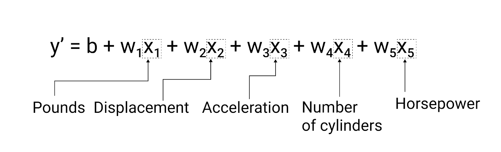
The goal in linear regression is to minimize the squared error consisting of all the data points:
We have several choices of loss functions for linear regression:

Regularization
Regularization is a technique to mitigate overfitting by penalizing noise through a parameter , with the purpose of trying to make a complex model (cause of overfitting) simpler.

The greater the parameter the more penalization there is for parameters being too large and that's how it makes a simpler model.
- small : If lambda is small then basically no regularization happens and the model retains its complexity
- large : If lambda is large, then large parameters get penalized and become smaller to avoid blowing up error and thus the model becomes simpler, increasing bias.
Here is an example of how one would undertake regularization:
- Perform k-fold cross validation with different values of .
- Choose the value that gave the lowest cross-validation error.
- Retrain on all the training data with the found value, and then test and see the generalization error.
Regularization punishes parameters to mitigate overfitting. By adding the parameters to the cost function, gradient descent aims to decrease the values of those parameters to make the hypothesis simpler.
There are three types of regularization:
- L1 regression: regularization using the norm
- L2 regression: regularization using the norm
- elastic regression: regularization combining both L1 and L2 regularization
| Effect | |
|---|---|
| L1 | Lasso regression is likely to completely reduce some parameters to 0, resulting in sparse models that require less memory. |
| L2 | Ridge regression reduces parameters a lot, but does not zero them out. |
| elastic | A healthy balance between L1 and L2 regularization |
Regularization fundamentals
Effect of regularization parameter
- As increases, the hypothesis becomes extremely more simple
- As decreases, the hypothesis becomes slightly more simple
A high value of penalizes the parameters a lot so that they are essentially 0, and the less that value, the less you are penalizing those parameters and thus the parameters only slightly decrease.
scaling
You must always scale data with any type of regression so that they can all be penalized the same without any skewed data.
NOTE
If data were not on the same scale, it would either grossly contribute to the cost or contribute nothing at all
regularization
regularization, also called lasso regression, sums up the absolute value (L1 norm) of all the parameters and adds that to the cost function
regularization
L2 regularization, also called ridge regression, sums up the squares (L2 norm) of all the parameters and adds that to the cost function.
Here is the cost function for ridge regression, which serves to add the beta coefficients to the cost function so that we can penalize them.
- : the number of training rows you have
- : the number of features/parameters
- : the regularization hyperparameter
Scaling
You must always scale data with ridge regression so that they can all be penalized appropriately.
- Scale training features
- Scale testing features with the same scaler parameters as you did for the training data.
ss = SS()
ss.fit(Xtrain)

# scale both training and testing data with scaler (based on training specs)
scaled_Xtrain = ss.transform(Xtrain)
scaled_Xtest = ss.transform(Xtest)
Hyperparameter optimization
Hyperparameter optimiziation is where we try to choose the best value for a hyperparameter that makes our model perform the best.
We always do hyperparameter optimization before training a model. Here are the steps we follow:
- Create a range for the values, like an array of hyperparameter values to test
- Loop through that range, and for each parameter, perform ridge regression with the regularization hyperparameter set to , and add that score to a list of model scores.
- Graph the alpha values against the list of model scores. THe optimal alpha lies at the peak of the graph.
from sklearn.preprocessing import StandardScaler as SS

def getOptimalAlpha() -> int :
    # 1. setup kfold and scaler
    k = 10
    ss = SS()

    # 2. create array of possible alpha values
    a_range = np.linspace(10,20,100)

    avg_tr_score=[]
    avg_te_score=[]

    for a in a_range:
        # 3. run model
        rid_reg = Ridge(alpha=a)
        train_scores, test_scores = do_Kfold(rid_reg, X, y, k, ss)

        # 4. collect statistics
        avg_tr_score.append(np.mean(train_scores))
        avg_te_score.append(np.mean(test_scores))

        # 5. return alpha that gave highest test score
        idx_max = np.argmax(avg_te_score)
        return a_range[idx_max]
K-nearest neighbors
Nearest Neighbor (NN)
The Nearest Neighbors (NN) algorithm works as follows:
- Represent a data point as a vector
- Given a data point, use the Euclidean distance formula with its vector representation to find its nearest neighbor, comparing to other data points.
- The neighbor with the least distance value to the data point will be considered as the nearest neighbor
Euclidean distance formula
This is how you describe the euclidean distance formula (or L2 norm) in any number of dimensions .
NOTE
The distance formula is just the same thing as subtracting the two vectors from each other and then taking the magnitude of that resultant vector.
KNN theory
The -Nearest Neighbors (-NN) algorithm is a non-parametric, instance-based supervised learning method that performs prediction by querying stored training data directly at test time without an explicit training phase.
-
Training Data Representation: The training set consists of pairs , where each is a -dimensional feature vector and is the target label.
- In classification,
- in regression, .
-
Core Assumption: Instances that are close to each other in feature space share the same or similar labels.
-
Lazy Learning: The algorithm requires computations at training time. It simply memorizes the entire dataset and defers all computation to test time.
To determine distance between data points, we use the L2 norm as the distance metric of choice, but there are multiple different distance metrics.
NN as KNN
-
1-NN (): Selects the single closest sample , and predicted label is directly assigned as .
-
-NN (): Finds the training examples having the smallest Euclidean distances to .
However, NN is naive because it is extremely sensitive to noise. KNN solves this problem by having more neighbors factor into a classification technique like majority voting.

Majority voting
The predicted label is determined by a plurality/majority vote among the neighbors:
Where is the indicator function:
NOTE
The main intuition here is that if most of the neighbors are in one category, then you join the majority category. For example, for if you have 6 neighbors in one category, the new data point gets labeled as part of that majority category
and the decision boundary
The choice of is a hyperparameter—a parameter that cannot be learned directly from training data and must be selected using a separate validation set.

| Parameter Choice | Model Behavior | Variance & Bias | Risk |
|---|---|---|---|
| Small (e.g., ) | Fits intricate local structures; captures fine-grained boundaries. Highly sensitive to label noise or outliers. | High Variance, Low Bias | Overfitting: Creates fragmented decision boundaries around mislabeled points. |
| Large (e.g., ) | Averages over broader neighborhoods; smooths out decision boundaries. | Low Variance, High Bias | Underfitting: Fails to capture localized patterns and may misclassify minority regions. |
-
Heuristic Guideline: A practical rule of thumb is to choose , where is the number of training samples.
-
Validation Strategy: Evaluate different candidate values of on a held-out validation set and pick the one with minimal validation error before performing final evaluation on the test set.

Distance metrics
In order to be a valid distance metric for KNN, it must satisfy three rules:
-
symmetric:
-
non-negative: The resulting distance must be non-negative
-
holds triangle inequality: When calculating a triangle of points, the triangle inequality must hold:
These distance metrics work for KNN:
- cosine similarity
- euclidean distance
- edit/hamming distances
The default distance metric for KNN is uniform, meaning every point is weighted equally. You can change this with the weights= kwarg when instantiating the KNN() object.
Distance metrics come into play when deciding how to tally up a positive prediction or a negative prediction from the k nearest points.
-
'uniform': Each point is weighted equally, no matter how far away it is from the data point. -
'distance': A point is weighted higher if it's closer to the data point being considered. Each point in the K nearest points to a data point is given a weight, which is the inverse of the distance from that point to the data point, 1 / distance.
KNN in implementation
In the k nearest neighbors algorithm, we choose a number , and in the corrdinate space, we consider a data point's distance to the nearest points to that data point.
Here are some things to keep in mind when implementing this algorithm in a ML practice:
- train vs test: For k nearest numbers, we want to keep train sets large and test sets small.
- scaling: Scaling is necessary for K nearest neighbors because this algorithm is dependent on the values of data points.
- distance metric: the choice of distance metric is crucial here.
- size of
- small k: Sensitive to noise, and overfits as a result
- large k: Takes into account too much data and underfits as a result.
NOTE
A good rule of thumb is to calculate
Scaling
Because Euclidean distance aggregates squared differences across all dimensions, features with larger numerical ranges (e.g., seconds vs. minutes, or kilograms vs. grams) disproportionately dominate the distance calculation.
Because KNN is based on distance, all the points must be on the same distance scale. Therefore something like standard scaling is necessary.
NOTE
For KNN classification, the neighbors approach only works if classes are not skewed. They need to be balanced, as in near 50-50, or else the neighbors approach will skew towards the majority class regardless of distance.
You can use standard scaling like so:
Transform each feature dimension to have zero mean and unit variance:
where is the mean and is the standard deviation of feature .
Runtime complexity
During training and testing, you don’t really make any computations while training. You only do computations when testing a point, which is ) complexity.
For each novel query instance at test time:
-
Distance Computations: arithmetic operations against all data points.
-
Neighbor Sorting: to rank distances and extract the top .
-
Space Complexity: memory to keep the complete training dataset loaded in RAM.
Code
In order to get the best performance of our model, we need to find out which value of k works best for the dataset. To fit a hyperparameter like k, we need to tune it on a validation set.
 The best way to do that is via KFOLD.
Code
-
Import
from sklearn.neighbors import KNeighborsClassifier as KNNfrom sklearn.preprocessing import StandardScaler as SS -
Create model
knn = KNN(n_neighbors=5) -
Fit model
knn.fit(X, y)
KNN() kwargs
n_neighbors=: the number of neighbors to set for the algorithm.weights=: changes the distance metric. Default is'uniform', where all points are weighted equally
Methods
knn.predict_proba(X): returns a soft classification for the features, giving probabilities for each classknn.predict(X): returns hard classification and classifies the observations to labels.knn.score(X, y): returns the accuracy of the model on the data
actual code
from sklearn.neighbors import KNeighborsClassifier as KNN
from sklearn.preprocessing import StandardScaler as SS
from sklearn.datasets import make_moons, make_blobs as mb, load_breast_cancer as lbc, load_iris as li
import pandas as pd
import numpy as np
import matplotlib.pyplot as plt
from sklearn.model_selection import train_test_split as tts
def knn_kfold(X, y, k):
neighbor_range = np.array(range(2,k))
train=[]
test=[]
# run through k nearest neighbord k times, doing k fold
for n_neighbors in neighbor_range:
knn = KNN(n_neighbors=n_neighbors)
tr, te = do_Kfold(knn, X, y, k, scaler=SS())
train.append(np.mean(tr))
test.append(np.mean(te))
# plot error against k
plt.figure(figsize=(6,6))
plt.plot(neighbor_range, train, ':xk', label='Training')
plt.plot(neighbor_range, test, ':xr', label='Testing')
plt.ylabel('Mean accuracy', fontsize=14)
plt.xlabel('$k$',fontsize=14)
plt.xticks(neighbor_range)
plt.legend()
plt.show()
KNN for regression and clustering
KNN is a non-parametric model, meaning that we don't really start off with a model equation like linear regression or a neural network we try to fit to per se, but rather we just let the algorithm do the work.
The main idea of the regression algorithm is this: for any new data point we will predict its target to be the average value of its k nearest neighbors and k is a hyperparameter we set for how many neighbors to check.
Over time this nudges data points even closer together and over thousands of iterations this eventually forms clusters, which helps you find categories and groupings via unsupervised learning.
Curse of dimensionality for KNN
K Nearest neighbors especially suffers whenever points in a space are roughly the same distance from each other, and in higher dimensionality, points are so dispersed from each other that they are approximately the same distance from each other due to the curse of dimensionality, so distance metrics become useless and unrepresentative.
As dimension grows, the volume of the feature space increases exponentially, causing data points to become extremely sparse.
Intrinsic dimensionality refers to the minimum number of parameters required to capture the essential characteristics of some data.
NOTE
K nearest neighbors works well on data with low intrinsic dimensionality like images.
-
the problem: In very high-dimensional spaces, distances between all pairs of points become roughly equidistant, eroding the predictive utility of proximity.
-
Saving Grace: Datasets like images often reside on or near a lower-dimensional manifold (a low intrinsic dimension), preserving meaningful neighborhood structures despite high raw dimensionality.
NOTE
TLDR
Due to how the curse of dimensionality makes data points in higher dimensions more equidistant, a distance-based algo like KNN suffers as a result. As number of features increases, k nearest neighbors becomes an increasingly worse algorithm
ML Engineering Primer
Best practices
Pick the right tool for the job
One of the most important parts of being an ML engineer is to always pick the right tool for the job. Different models excel in different areas and you need to pick the one that makes sense for the business problem.
-
Structured/Tabular Operational Data: If you are predicting administrative workflow durations, resource bottlenecks, or classification tasks on structured database logs, classical ML (like Gradient Boosted Trees via XGBoost/LightGBM or regularized logistic regression) often outperforms LLMs, trains in seconds, costs fractions of a cent, and offers native feature importance (explainability).
-
Unstructured Text & Reasoning: When dealing with unstructured documents, policy manuals, or complex semantic parsing, Large Language Models and retrieval pipelines shine.
Each tool has its tradeoffs, which you can classify in 4 core areas:
-
Cost: Inference costs at scale compound quickly with LLMs. Token efficiency matters.
-
Latency: Real-time administrative tools need sub-second or low-latency responses. Heavy models or multi-step agent loops introduce bottlenecks.
-
Reliability & Determinism: Classical models are mathematically deterministic. LLMs are probabilistic—requiring guardrails (e.g., JSON mode, function calling, or programmatic constraints).
-
Explainability: In institutional or operational environments, stakeholders often need to know why a decision or prediction was made.
Here's an appropriate interview response to feign expertise:
"When approaching a problem for the Accelerator team, I treat model selection as an architectural trade-off. If we're automating structured operational routing, a gradient-boosted tree gives us high performance, low latency, and native feature interpretability at minimal cost. If we're parsing unstructured administrative policies to automate workflows, that's when we lean into LLMs coupled with rigorous evaluation guardrails."
Evaluating models
1. Pre-Deployment (Offline) Evaluation
Before any model or agent touches production, you must evaluate it against a curated test dataset of edge cases and ground-truth expectations.
-
Classical ML Metrics: Precision, recall, -score, ROC-AUC, and calibration curves to ensure your probabilities match reality.
-
LLM & RAG Evaluation (e.g., using frameworks like Ragas or TruLens):
-
Context Precision & Recall: Did the retrieval system actually fetch the right internal documents?
-
Faithfulness / Groundedness: Is the model's generated answer strictly derived from the retrieved context, or is it hallucinating?
-
Answer Relevance: Did it actually answer the user's prompt without introducing off-topic noise?
-
Observability & Monitoring against drift and bias
Bias is seen when predictions are less favorable to an individual or group.
Model drift happens when the relationship between the target variable and other input variables changes over time after the model is deployed, and can introduce bias in your model after production.
- This means the patterns the model learned during training no longer fully apply, causing its predictions to become less accurate.
- Drift can occur due to changes in real-world data or environment where the model operates.
Once in production, static metrics degrade because the real world changes. You must monitor for two primary types of drift:
-
Data Drift: The statistical properties of incoming input data change over time (e.g., users writing administrative requests using entirely new terminology or formatting).
-
Concept Drift: The statistical relationship between the input and the target output changes (e.g., an internal approval policy changes, making previous historical routing logic obsolete).
-
Operational Metrics: Latency (p95/p99), token consumption/cost tracking, and error/exception rates.
Here are the different ways to mitigate drift:
- feature engineering: one approach is weighting important features so the model focuses more on stable, relevant data points. Understanding and managing drift is key to keeping machine learning models reliable in production.
3. Rigorous Experimentation
- A/B Testing: Routing a percentage of live production traffic to a newly fine-tuned model or updated prompt chain to measure concrete business impact (e.g., resolution time, user correction rate) before full rollout.
ML pipeline
A machine learning pipeline is a way to organize and automate all the steps involved in building a machine learning model—from preparing data, training the model, evaluating it, tuning parameters, to deploying it.
Instead of running each step separately, a pipeline groups them into a single, streamlined process.
NOTE
Pipelines make your workflow more efficient, reproducible, and easier to manage.
Here are the key benefits:
- have parallelization capability: Pipelines also speed up training by running tasks in parallel and help ensure consistent data preparation across different model training runs.
- reliability and reproducibility: This approach is especially helpful in production environments where you want reliable and maintainable ML systems.

Sci-kit learn pipeline
Here's an example pipeline:
- Get data
import sklearn
from sklearn.model_selection import train_test_split

# remove spaces from column names and convert all to lowercase and remove special characters as it could cause issues in the future
housing_df_encoded.columns = [c.lower().replace(' ', '_').replace('<', '_') for c in housing_df_encoded.columns]

# Split target variable and feature variables
X = housing_df_encoded[['housing_median_age', 'median_income','bedrooms_per_room','population_per_household','coords','ocean_proximity__1h_ocean',
                        'ocean_proximity_inland','ocean_proximity_island','ocean_proximity_near_bay','ocean_proximity_near_ocean']]
y = housing_df_encoded['median_house_value']

X_train, X_test, y_train, y_test = train_test_split(X, y, random_state=42, shuffle=True, test_size=0.3)
- Create pipeline
from sklearn.pipeline import Pipeline
from sklearn.linear_model import LinearRegression
from sklearn.ensemble import RandomForestRegressor
from xgboost import XGBRegressor


pipeline_lr= Pipeline([('lr_classifier', LinearRegression())])
pipeline_rf = Pipeline([('rf_classifier', RandomForestRegressor(n_estimators=10,random_state=10))])
pipeline_xgb = Pipeline([('xgb_classifier', XGBRegressor())])

pipelines = [pipeline_lr, pipeline_rf, pipeline_xgb]
pipe_dict = {0: 'Linear Regression', 1: 'Random Forest Regressor', 2: 'XGBRegressor'}

for pipe in pipelines:
    pipe.fit(X_train, y_train)

for i,model in enumerate(pipelines):
    pred_test = model.predict(X_test)
    if i == 1: rf_model = model
    print("{} Test Accuracy:{}".format(pipe_dict[i],model.score(X_test,y_test)))
    print(pd.DataFrame({'Actual': y_test, 'Predicted': pred_test}))